## Uncomment for colab users
# !pip install amtutorialEnergy Transformer
Rederiving the Transformer as an energy-based Associative Memory.
![]()
Flow perspective of Transformers
Squint, and the Transformer looks like a dynamical system.
At its core, the transformer is a stack of \(L\) transformer blocks that takes a length \(N\) sequence of input tokens \(\{\mathbf{x}^{(0)}_1, \ldots, \mathbf{x}^{(0)}_N\}\) and outputs a length \(N\) sequence of output tokens \(\{\mathbf{x}^{(L)}_1, \ldots, \mathbf{x}^{(L)}_N\}\). Each token \(\mathbf{x}^{(l)}_i \in \mathbb{R}^D\) is a vector of dimension \(D\).
When blocks are stacked, the residual connections form a “residual highway” that consists entirely of normalizations and additions from Attention and MLP operations.
Associative Memory (AM) requires a global energy function, where each computation minimizes the total energy of the system. Our goal is to derive an energy function whose gradient looks as much like the Transformer block as possible.
Introducing Energy into the Transformer
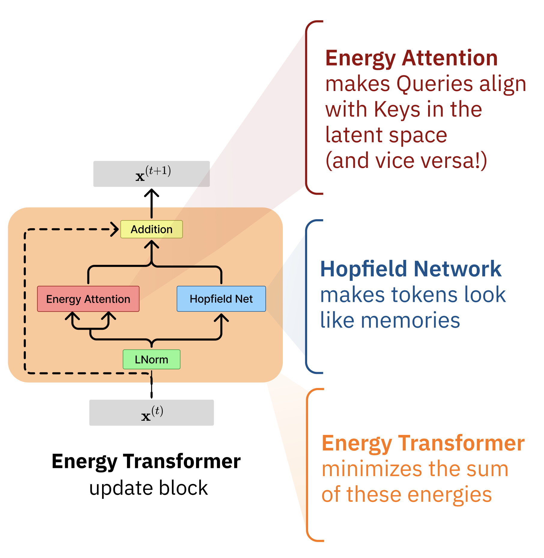
We will now build a kind of associative memory called the “Energy Transformer” [1] that turns the familiar transformer operation into an energy minimization. Energy Transformer (ET) defines a single energy on an \(\mathbf{x} \in \mathbb{R}^{N \times D}\) collection of tokens, where we can think of each token \(\mathbf{x}_B\) as a “particle” that knows some information about itself and needs to figure out what it should become. Some particles (unmasked tokens) already know their identity, while others (masked tokens) only know their position and must discover their identity by interacting with their neighbors.
Minimizing the energy of the Energy Transformer (ET) is a recurrent process. The entire transformer consists of a single Transformer block, and each “layer” of the transformer becomes a gradient descent step down the energy. This gradient descent step looks remarkably like a standard transformer block, complete with attention, MLP-like operations, layer normalizations, and residual connections.
The global energy combines two intuitive ideas: (1) attention energy that encourages masked tokens to align with relevant unmasked tokens, and (2) memory energy that ensures all tokens look like realistic patterns the model has learned. The gradient of each of these energies look like a self-attention and MLP, respectively, with some shared weight constraints.
This is one of those situations where the code ends up being significantly simpler than the equations. We write the equations for completeness, but feel free to skip to Section 2.3 for succinct code.
Attention Energy
We describe the energy of a multi-headed attention with \(H\) heads, where the \(h\)-th head of attention is parameterized by \(\mathbf{W}_h^Q, \mathbf{W}_h^K \in \mathbb{R}^{D \times Y}\), where \(Y\) is the “head dimension”. The input to the attention is the normalized token vectors \(\hat{\mathbf{x}} \in \mathbb{R}^{N \times D}\). In the math that follows, we index the heads by \(h=1\ldots H\), the head dimension by \(\alpha=1\ldots Y\), tokens by \(A,B,C=1 \ldots N\), and each token vector by \(i,j=1\ldots D\).
Einstein notation
We find it convenient to use Einstein notation for the math, since it maps 1:1 to the einops operations we’ll use in the code. If you aren’t familiar with the notation, check out this awesome tutorial. But fair warning, the equations at first look pretty complicated with all the indices.
One tip for reading equations with lots of indices: you don’t need to remember the shape or order of tensors, just remember the meaning of the indices. The number of subscripts is the number of dimensions of the tensor, and the meaning of each dimension is captured in the index name. For example, let \(B=1\ldots N\) index the token position in a sequence, and let \(i=1\ldots D\) index into each token vector. \(x_{Bi}\) is an element of a 2-dimensional tensor capturing the sequence length \(N\) and token dimension \(D\). Transposes don’t have meaning since things are named, so \(x_{Bi} = x_{iB}\). So long as you know the index semantics, you can read always read the equation. Everything is just scalar multiplication and addition.
The familiar queries and keys are computed as normal linear transformations:
\[ \begin{split} K_{h \alpha B} &= \sum\limits_j W^K_{h \alpha j}\; \hat{x}_{Bj}, \qquad \mathbf{K} \in \mathbb{R}^{H \times Y \times N} \\ Q_{h \alpha C} &= \sum\limits_j W^Q_{h \alpha j}\; \hat{x}_{Cj}, \qquad \mathbf{Q} \in \mathbb{R}^{H \times Y \times N} \end{split} \]
Our familiar “raw attention scores” (pre-softmax) are still the dot-product correlations between each query and key:
\[ A_{hBC} = \sum_{\alpha} K_{h\alpha B} Q_{h\alpha C} \]
Now for the different part: we describe the energy of the attention as the negative log-sum-exp of the attention scores. We will use the \(\beta\) as an inverse-temperature hyperparameter to scale the attention scores.
\[ E^\text{ATT} = -\frac{1}{\beta} \sum_{h=1}^H \sum_{C=1}^N \log \left( \sum_{B \neq C} \exp(\beta A_{hBC}) \right) \tag{1}\]
As we saw in a previous notebook, the negative log-sum-exp is an exponential variation of the Dense Associative Memory. The cool thing is that the gradient of the negative log-sum-exp is the softmax, which is what we’d like to see in the attention update rule.
Where are our values?
You may recall that traditional attention also has a value matrix. When we take the gradient of Equation 1, we lose the flexibility to include an independently parameterized values: the values must be a function of the queries and the keys.
Memory Energy
In traditional transformers, the MLP (without biases) can be written as a two-layer feedforward network with a ReLU on the hidden activations. The MLP is parameterized by two weight matrices \(\mathbf{V}, \mathbf{W} \in \mathbb{R}^{M \times D}\) where \(M\) is the size of the hidden layer (\(M=4D\) is often viewed as the default expansion factor atop token dimension \(D\)). Let’s again use Einstein notation, where \(\mu=1\ldots M\) indexes the hidden units, \(i,j=1\ldots D\) index the token dimensions, and \(B=1\ldots N\) indexes each token.
\[ \text{MLP}(\hat{\mathbf{x}})_{Bi} = \sum_\mu W_{\mu i} \; \text{ReLU}\left(\sum_j V_{\mu j} \hat{\mathbf{x}}_{Bj}\right) \tag{2}\]
If we assume weight sharing between \(\mathbf{V} = \mathbf{W} = \boldsymbol{\xi}\), this is a gradient descent step down the energy of a Hopfield Network
\[ E^{\text{HN}}(\hat{\mathbf{x}}) = - \sum_{B, \mu} F\left(\sum_j \xi_{\mu j} \hat{\mathbf{x}}_{Bj}\right) \]
with rectified quadratic energy \(F(\cdot) := \frac12 \text{ReLU}(\cdot)^2\). If we say \(f(\cdot) := F'(\cdot) = \text{ReLU}(\cdot)\), the negative gradient of the energy is
\[ -\frac{\partial E^{\text{HN}}(\mathbf{\hat{x}})}{\partial \hat{x}_{Bi}} = \sum_\mu \xi_{\mu i} \; f\left(\sum_j \xi_{\mu j} \hat{\mathbf{x}}_{Bj}\right), \]
which is identical to the MLP operation in Equation 2 with a weight sharing constraint.
Note
It is perfectly reasonable to consider other convex functions \(F\) for use in the energy. Polynomials of higher degree \(n\) or exponential functions are both valid and will yield Dense Associative Memory. However, because traditional Transformers use a ReLU activation, we use a rectified quadratic energy.
ET in code
Let’s implement the attention energy in code. We will use jax and equinox for our code.
Necessary imports
import jax, jax.numpy as jnp, jax.random as jr, jax.tree_util as jtu, jax.lax as lax
import equinox as eqx
from dataclasses import dataclass
from typing import *
import matplotlib.pyplot as plt
import numpy as np
import imageio.v2 as imageio
from glob import glob
from fastcore.basics import *
from fastcore.meta import *
import matplotlib.pyplot as plt
from jaxtyping import Float, Array
import functools as ft
from einops import rearrange
from amtutorial.data_utils import get_et_imgs, get_et_checkpoint
The EnergyTransformer class captures all the token processing in the entire transformer. There are maybe 7 lines of code that perform the actual energy computation. This single energy function, when paired with a layer-norm, is analogous to the full computation across all layers of a traditional transformer. The only things missing are some some token and position embedding matrices to make it work on real data, but we will do that in the following section.
First, let’s describe the configuration for ET:
class ETConfig(eqx.Module):
  D: int = 768 # token dimension
  H: int = 12 # number of heads
  Y: int = 64 # head dimension
  M: int = 3072 # MLP size
  beta: Optional[float] = None # Inverse temperature for attention, defaults to 1/sqrt(Y)
  prevent_self_attention: bool = True # Prevent explicit self-attention
  def get_beta(self): return self.beta or 1/jnp.sqrt(self.Y)

smallETConfig = ETConfig(D=12, H=2, Y=6, M=24)
mediumETConfig = ETConfig(D=128, H=4, Y=32, M=256)
fullETConfig = ETConfig(D=768, H=12, Y=64, M=3072, beta=1/jnp.sqrt(64))
The ETConfig class captures all the dimensions and default hyperparameters for ET. The only thing left to do is implement the energies of Energy Transformer
class EnergyTransformer(eqx.Module):
  config: ETConfig
  Wq: Float[Array, "H D Y"] # Query projection
  Wk: Float[Array, "H D Y"] # Key projection
  Xi: Float[Array, "M D"]
EnergyTransformer is parameterized by only three matrices: \(\mathbf{W}^Q, \mathbf{W}^K\) and \(\mathbf{Xi}\) (we did not choose to introduce any biases, though we could have).
We use these parameters to define both the attention energy and the memory energy.
@patch
def attn_energy(self: EnergyTransformer, xhat: Float[Array, "N D"]):
  beta = self.config.get_beta()
  K = jnp.einsum("kd,hdy->khy", xhat, self.Wk)
  Q = jnp.einsum("qd,hdy->qhy", xhat, self.Wq)
  N = K.shape[0]
  if self.config.prevent_self_attention:
    bmask = jnp.ones((N, N)) - jnp.eye(N) # Prevent self-attention
  else:
    bmask = jnp.ones((N, N))
  A = jax.nn.logsumexp(beta * jnp.einsum("khy,qhy->hqk", K, Q), b=bmask, axis=-1)
  return -1/beta * A.sum()

@patch
def hn_energy(self: EnergyTransformer, xhat: Float[Array, "N D"]):
  """ReLU-based "memory energy" using a Hopfield Network"""
  hid = jnp.einsum("nd,md->nm", xhat, self.Xi)
  return -0.5 * (hid.clip(0) ** 2).sum()
The total energy is just the sum of the attention and memory energies.
@patch
def energy(self: EnergyTransformer, xhat: Float[Array, "N D"]):
  "Total energy of the Energy Transformer"
  return self.attn_energy(xhat) + self.hn_energy(xhat)
And finally, let’s make a classmethod to easily initialize the module with random parameters.
@patch(cls_method=True)
def rand_init(cls: EnergyTransformer, key, config: ETConfig):
  key1, key2, key3 = jr.split(key, 3)
  return cls(config,
    Wq=jr.normal(key1, (config.H, config.D, config.Y)) / jnp.sqrt(config.Y),
    Wk=jr.normal(key2, (config.H, config.D, config.Y)) / jnp.sqrt(config.Y),
    Xi=jr.normal(key3, (config.M, config.D)) / jnp.sqrt(config.D)
  )
Special Layer Normalization
Note that the xhat inputs above are all layer-normalized tokens. However, like other AMs, we restrict ourselves to using non-linearities that are gradients of a convex Lagrangian function. Our “special layernorm” is the same as the standard layer normalization except that we need our learnable gamma parameter to be a scalar instead of a vector of shape D. We will just show this in code below.
class EnergyLayerNorm(eqx.Module):
  """Define our primary activation function (modified LayerNorm) as a lagrangian with energy"""
  gamma: Float[Array, ""]  # Scaling scalar
  delta: Float[Array, "D"] # Bias per token
  use_bias: bool = False
  eps: float = 1e-5

  def lagrangian(self, x):
    """Integral of the standard LayerNorm"""
    D = x.shape[-1]
    xmeaned = x - x.mean(-1, keepdims=True)
    t1 = D * self.gamma * jnp.sqrt((1 / D * xmeaned**2).sum() + self.eps)
    if not self.use_bias: return t1
    t2 = (self.delta * x).sum()
    return t1 + t2

  def __call__(self, x):
    """LayerNorm. The derivative of the Lagrangian"""
    xmeaned = x - x.mean(-1, keepdims=True)
    v = self.gamma * (xmeaned) / jnp.sqrt((xmeaned**2).mean(-1, keepdims=True)+ self.eps)
    if self.use_bias: return v + self.delta
    return v
That’s it! We rely on autograd to do the energy minimization, or the “inference” pass through the entire transformer.
Let’s check that the energy both monotonically decreases and is bounded from below.
key = jr.PRNGKey(11)
et = EnergyTransformer.rand_init(key, config=smallETConfig)
lnorm = EnergyLayerNorm(gamma=1., delta=jnp.zeros(et.config.D))

def energy_recall(Efn, x_init, nsteps, step_size):
  "Simple gradient descent to recall a memory"
  @jax.jit
  def gd_step(x, i):
      energy, grad = jax.value_and_grad(Efn)(lnorm(x))
      x_next = x - step_size * grad
      return x_next, energy

  xhat_init = lnorm(x_init)
  final_x, energy_history = jax.lax.scan(
      gd_step,
      xhat_init,
      jnp.arange(nsteps)
  )
  return final_x, energy_history

x_init = jr.normal(key, (100, et.config.D)) # Layer normalized tokens
final_x, energy_history = energy_recall(et.energy, x_init, nsteps=3000, step_size=0.5)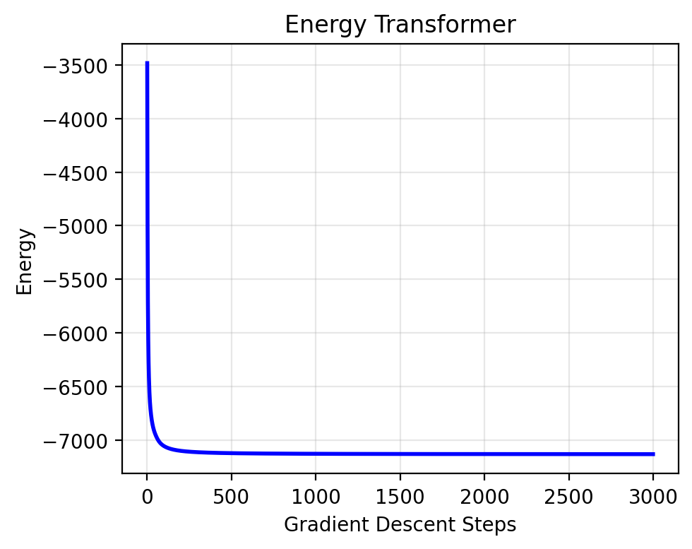
Inference with an Energy Transformer
To make the Energy Transformer described above work on real data, we need to add some necessary addendums to work with image data: the token and position embedding matrices, and some data processing code.
Loading data
Energy Transformer was originally trained on ImageNet. We will load some example images (unseen during training) to demonstrate ET’s ability to remember images.
# Load and prepare unseen images
IMAGENET_MEAN = np.array([0.485, 0.456, 0.406]) * 255 # C, H, W
IMAGENET_STD = np.array([0.229, 0.224, 0.225]) * 255 # C, H, W

def normalize_img(im):
  """Put into channel first format, normalize"""
  x = (im - IMAGENET_MEAN) / IMAGENET_STD
  x = rearrange(x, "h w c-> c h w")
  return x

def unnormalize_img(x):
  """Put back into channel last format, denormalize"""
  x = rearrange(x, "c h w -> h w c")
  im = (x * IMAGENET_STD) + IMAGENET_MEAN
  return im.astype(jnp.uint8)

@ft.lru_cache
def get_normalized_imgs():
  imgs = jnp.array(get_et_imgs())
  imgs = jax.vmap(normalize_img)(imgs)
  return imgs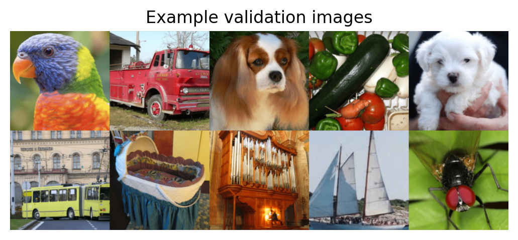
Patching images
We build a Patcher class to patchify and unpatchify images, which is mostly a simple wrapper around the rearrange function from einops.
Patcher class
class Patcher(eqx.Module):
  "Patchify and unpatchify an image."
  image_shape: Iterable[int] # (C, H, W) Image shape
  patch_size: int # Square patch size
  kh: int # Number of patches in the height direction
  kw: int # Number of patches in the width direction

  @property
  def patch_shape(self): return (self.image_shape[0], self.patch_size, self.patch_size)

  @property
  def num_patch_elements(self): return ft.reduce(lambda a, b=1: a * b, self.patch_shape)

  @property
  def num_patches(self): return self.kh * self.kw

  def patchify(self, img):
    "Turn an image (possibly batched) into a collection of patches."
    return rearrange(
      img,
      "... c (kh h) (kw w)-> ... (kh kw) c h w",
      h=self.patch_size,
      w=self.patch_size,
    )

  def unpatchify(self, patches):
    "Turn a collection of patches (possibly batched) back into an image."
    return rearrange(
      patches, "... (kh kw) c h w -> ... c (kh h) (kw w)", kh=self.kh, kw=self.kw
    )

  def rasterize(self, patches):
    "Rasterize patches into tokens"
    return rearrange(patches, "... c h w -> ... (c h w)")

  def unrasterize(self, tokens):
    "Unrasterize tokens into patches"
    c,h,w = self.patch_shape
    return rearrange(tokens, "... (c h w) -> ... c h w", c=c, h=h, w=w)

  def tokenify(self, img):
    "Turn img into rasterized patches"
    return self.rasterize(self.patchify(img))

  def untokenify(self, tokens):
    "Untokenify tokens into original image"
    return self.unpatchify(self.unrasterize(tokens))

  def patchified_shape(self):
    "The expected shape of a patchified image"
    return (self.num_patches, *self.patch_shape)

  @classmethod
  def from_img(cls, img, patch_size):
    "Create a Patcher from an example image."
    return cls.from_img_shape(img.shape, patch_size)

  @classmethod
  def from_img_shape(cls, img_shape, patch_size):
    "Create a patcher from a specified image shape."
    height, width = img_shape[-2:]
    assert (height % patch_size) == 0
    assert (width % patch_size) == 0
    kh = int(height / patch_size)
    kw = int(width / patch_size)
    return cls(img_shape, patch_size, kh, kw)
It lets us do things like:
patcher = Patcher.from_img_shape(imgs[0].shape, patch_size=16)
patched_img = patcher.patchify(imgs[0])
print(patched_img.shape)
(196, 3, 16, 16)RuntimeWarning: invalid value encountered in cast
return im.astype(jnp.uint8)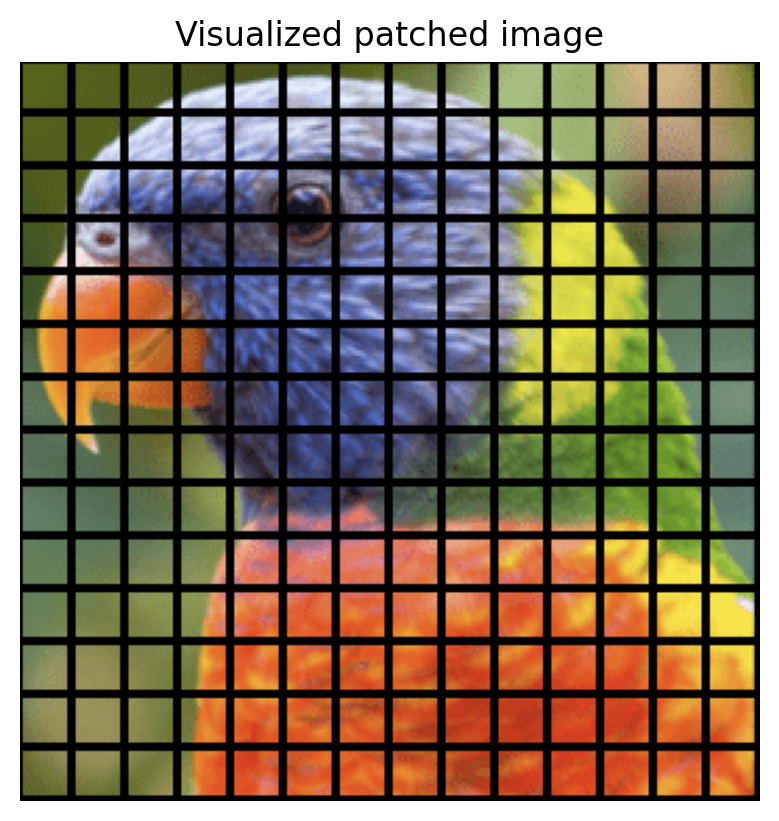
Patcher.unpatchify gets us back to the original image.
assert jnp.all(patcher.unpatchify(patched_img) == imgs[0])We can also process an images and batches of imags into tokens and back.
tokenified_img = patcher.tokenify(imgs[0])
print("Token pre-embedding shape: ", tokenified_img.shape)

untokenified_img = patcher.untokenify(tokenified_img)
assert jnp.all(untokenified_img == imgs[0])

batch_tokenified_imgs = patcher.tokenify(imgs)
print("Batch token pre-embedding shape: ", batch_tokenified_imgs.shape)

batch_untokenified_imgs = patcher.untokenify(batch_tokenified_imgs)
assert jnp.all(batch_untokenified_imgs == imgs)
Token pre-embedding shape: (196, 768)
Batch token pre-embedding shape: (11, 196, 768)Image-compatible ET
Let’s create a full ET, complete with embeddings, model that can be used for masked-image inpainting. We say that each image has \(N\) total patches/tokens, where each patch as \(Z = c \times h \times w\) pixels when rasterized. We will use linear embeddings (with biases) to embed and unembed rasterized image patches to tokens.
First, let’s describe the data and ET we are working with.
class ImageETConfig(eqx.Module):
  image_shape: Tuple[int, int, int] = (3, 224, 224) # (C, H, W) Image shape
  patch_size: int = 16 # Square patch size
  et_conf: ETConfig = fullETConfig
To work with data, we add a few extra matrices: embedding/unembedding matrices (let’s use a bias for each), position embeddings, and CLS/MASK tokens. The position embeddings are used to encode the position of each token in the sequence, and the CLS/MASK tokens are used for interop with the original ViT. [2] Additionally, the layernorm is external to the computation of the ET so we’ll insert those parameters here.
class ImageEnergyTransformer(eqx.Module):
  patcher: Patcher
  W_emb: Float[Array, "Z D"]
  b_emb: Float[Array, "D"]
  W_unemb: Float[Array, "D Z"]
  b_unemb: Float[Array, "Z"]

  pos_embed: Float[Array, "(N+1) D"] # Don't forget the CLS token!
  cls_token: jax.Array
  mask_token: jax.Array
  et: EnergyTransformer
  lnorm: EnergyLayerNorm

  config: ImageETConfig
Let’s define some functions for converting image patches to/from tokens. These are a.k.a. “embedding” and “unembedding” operations.
@patch
def encode(
  self: ImageEnergyTransformer,
  x: Float[Array, "N Z"]
):
  "Embed rasterized patches to tokens"
  out = x @ self.W_emb + self.b_emb # (..., N, D)
  return out

@patch
def decode(
  self: ImageEnergyTransformer,
  x: Float[Array, "N D"]):
  "Turn x from tokens to rasterized img patches"
  return x @ self.W_unemb + self.b_unemb # (..., N, Z)
Masking tokens is also a part of this data connection. Let’s corrupt and add the CLS register:
@patch
def corrupt_tokens(
  self: ImageEnergyTransformer,
  x: Float[Array, "N D"],
  mask: Float[Array, "N"],
  max_n_masked: int=100):
  """Corrupt tokens with MASK tokens wherever `mask` is 1.

  `max_n_masked` needs to be known in advance for JAX JIT to work properly
  """
  maskmask = jnp.nonzero(mask == 1, size=max_n_masked, fill_value=0)
  return x.at[maskmask].set(self.mask_token) # (..., N, D)

@patch
def prep_tokens(
  self: ImageEnergyTransformer,
  x: Float[Array, "N D"],
  mask: Float[Array, "N"]):
  "Add CLS+MASK tokens and POS embeddings"
  x = self.corrupt_tokens(x, mask)
  x = jnp.concatenate([self.cls_token[None], x]) # (..., N+1, D)
  return x + self.pos_embed # (..., N+1, D)
The inference process is gradient descent down the energy, and turns a full image whose patches are masked according to mask and returns predictions for the whole image.
@patch
def __call__(
  self: ImageEnergyTransformer,
  img: Float[Array, "C H W"],
  mask: Float[Array, "N"],
  nsteps=12,
  step_size=0.1):
  "A complete pipeline for masked image modeling in ET using gradient descent"
  x = self.patcher.tokenify(img) # (..., N, Z)
  x = self.encode(x)
  x = self.prep_tokens(x, mask)  # (..., N+1, D)

  get_energy_info = jax.value_and_grad(self.et.energy)

  def gd_step(x, i):
      xhat = self.lnorm(x)
      E, dEdg = get_energy_info(xhat)
      x_next = x - step_size * dEdg
      return x_next, {"energy": E, "xhat": xhat}

  x, traj_outputs = jax.lax.scan(gd_step, x, jnp.arange(nsteps))

  xhat_final = self.lnorm(x)
  E_final = self.et.energy(xhat_final)
  traj_outputs['xhat'] = jnp.concatenate([traj_outputs['xhat'], xhat_final[None]], axis=0)
  traj_outputs['energy'] = jnp.concatenate([traj_outputs['energy'], E_final[None]], axis=0)

  xhat_final = xhat_final[1:]  # Discard CLS token for masked inpainting
  x_decoded = self.decode(xhat_final)
  return self.patcher.untokenify(x_decoded), traj_outputs
Random initialization helper
For completeness, let’s add a helper function to initialize the model with random parameters. We won’t use it in this tutorial, however.
@patch(cls_method=True)
def rand_init(cls: ImageEnergyTransformer, key, config=ImageETConfig()):
  key1, key2, key3, key4, key5, key6, key7, key8 = jr.split(key, 8)
  patcher = Patcher.from_img_shape(config.image_shape, config.patch_size)
  W_emb = jr.normal(key1, (patcher.num_patch_elements, config.et_conf.D)) / config.et_conf.D
  b_emb = jr.normal(key2, (config.et_conf.D,))
  W_unemb = jr.normal(key3, (config.et_conf.D, patcher.num_patch_elements)) / patcher.num_patch_elements
  b_unemb = jr.normal(key4, (patcher.num_patch_elements,))
  pos_embed = jr.normal(key5, (patcher.num_patches, config.et_conf.D)) / config.et_conf.D
  cls_token = 0.002 * jr.normal(key6, (config.et_conf.D,))
  mask_token = 0.002 * jr.normal(key7, (config.et_conf.D,))
  pos_embed = 0.002 * jr.normal(key8, (1 + patcher.num_patches, config.et_conf.D)) / config.et_conf.D

  return cls(
    patcher=patcher,
    W_emb=W_emb,
    b_emb=b_emb,
    W_unemb=W_unemb,
    b_unemb=b_unemb,
    pos_embed=pos_embed,
    cls_token=cls_token,
    mask_token=mask_token,
    et=EnergyTransformer.rand_init(key7, config.et_conf),
    lnorm=EnergyLayerNorm(gamma=1., delta=jnp.zeros(config.et_conf.D)),
    config=config
  )

imageET = ImageEnergyTransformer.rand_init(key, ImageETConfig())
Loading pretrained weights
ET has publicly available pretrained weights that can be used for masked-image inpainting. The model itself is pretty small ~20MB, with no compression tricks on the weights (everything is np.float32). We load the state dict from a saved .npz file as follows:
@ft.lru_cache
def get_pretrained_et():
  load_dict = {k: jnp.array(v) for k,v in get_et_checkpoint().items()}

  # config from state_dict
  H, Y, D = load_dict["Wk"].shape
  D, M = load_dict["Xi"].shape

  et_config = ETConfig(D=D, H=H, Y=Y, M=M, prevent_self_attention=False) # These weights were trained allowing self attention. But the arch works equally well both ways.
  et = EnergyTransformer(
    Wk = rearrange(load_dict["Wk"], "h y d -> h d y"),
    Wq = rearrange(load_dict["Wq"], "h y d -> h d y"),
    Xi = rearrange(load_dict["Xi"], "d m -> m d"),
    config = et_config
  )

  image_config = ImageETConfig(image_shape=(3, 224, 224), patch_size=16, et_conf=et_config)
  patcher = Patcher.from_img_shape(image_config.image_shape, image_config.patch_size)
  iet = ImageEnergyTransformer(
    patcher = patcher,
    W_emb = load_dict["Wenc"],
    b_emb = load_dict["Benc"],
    W_unemb = load_dict["Wdec"],
    b_unemb = load_dict["Bdec"],
    pos_embed = load_dict["POS_embed"],
    cls_token = load_dict["CLS_token"],
    mask_token = load_dict["MASK_token"],
    et = et,
    lnorm = EnergyLayerNorm(gamma=load_dict["LNORM_gamma"], delta=load_dict["LNORM_bias"]),
    config = image_config
  )

  return iet
We can inpaint images with ET.
def inpaint_image(
  iet: ImageEnergyTransformer,
  img: Float[Array, "C H W"],
  n_mask: int,
  key: jax.random.PRNGKey,
  nsteps: int=12,
  step_size: float=0.1):
    " Perform masked image inpainting with Energy Transformer"
    # Create random mask
    mask_idxs = jr.choice(
        key, np.arange(iet.patcher.num_patches), shape=(n_mask,), replace=False
    )
    mask = jnp.zeros(iet.patcher.num_patches).at[mask_idxs].set(1)

    x = iet.patcher.tokenify(img)
    x = iet.encode(x)  # Img to embedded tokens
    x = iet.prep_tokens(x, mask)[1:]  # N,D (remove CLS token)
    masked_img = iet.decode(iet.lnorm(x))
    masked_img = iet.patcher.untokenify(masked_img)

    # Reconstruct image using Energy Transformer
    recons_img, traj_outputs = iet(img, mask, nsteps=nsteps, step_size=step_size)

    return masked_img, recons_img, traj_outputs

iet = get_pretrained_et()
nh, nw = 2, 5
N = nh*nw
og_imgs = get_normalized_imgs()[:N]

keys = jr.split(jr.PRNGKey(0), len(og_imgs))
masked_imgs, recons_imgs, traj_outputs = jax.vmap(inpaint_image, in_axes=(None, 0, None, 0))(iet, og_imgs, 100, keys)

vunnormalize_img = jax.vmap(unnormalize_img)
og_imgs_show, masked_imgs_show, recons_imgs_show = [vunnormalize_img(im) for im in (og_imgs, masked_imgs, recons_imgs)]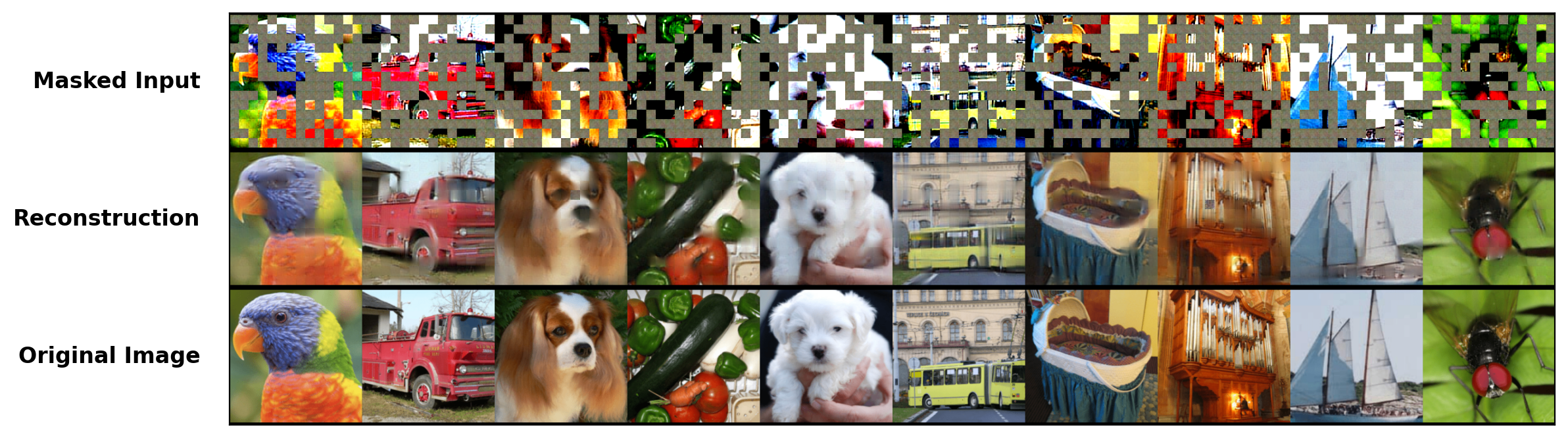
We can also animate the retrieval.
Animation dependencies
from pathlib import Path
import matplotlib.animation as animation
from IPython.display import Video, Markdown
from moviepy.editor import ipython_display
import os

CACHE_DIR = Path("./cache") / "01_energy_transformer"
CACHE_DIR.mkdir(exist_ok=True, parents=True)
CACHE_VIDEOS = TrueThese images are fully reconstructed using autograd down the parameterized energy function. You may notice the reconstructions are not perfect, e.g., the right eye of the white dog is missing.
The energy is still decreasing! Shouldn’t the images get better if we run longer?
Unfortunately, these weights were only trained to 12 steps at a fixed step size. Running longer will still cause the energy to decrease, but our image reconstruction quality will not improve. This reflects that our model has learned a kind of ‘metastable state’ at which nice reconstructions are retrieved, but these reconstructions are not “memories” in the formal definition of the term.
masked_imgs, recons_imgs, traj_outputs = jax.vmap(ft.partial(inpaint_image, nsteps=40), in_axes=(None, 0, None, 0))(iet, og_imgs, 100, keys)
video, video_fname = show_et_recall_animation(iet, traj_outputs, "et_reconstruction_long",
steps_per_sample=1, force_remake=True)Interpreting ET
The representations learned by ET are attractors of the dynamics. That is, the weights of the Hofield Network in ET are not arbitrary linear transformations — they are actual stored data patterns. Visualizing the weights reveals what the model has actually learned.
def decode_stored_pattern(iet, xi):
  c,h,w = iet.patcher.patch_shape
  decoded = iet.decode(iet.lnorm(xi))
  patches = rearrange(decoded, '... (c h w) -> ... c h w', c=c, h=h, w=w)
  return unnormalize_img(patches)

Xi_show = jax.vmap(ft.partial(decode_stored_pattern, iet))(iet.et.Xi)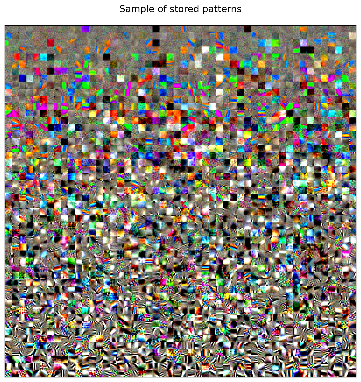
Interpretability by design
You can think of the Hopfield Network like an SAE that is integrated into the core computation of the model. Interpretability is a natural byproduct of good architecture design.
References
[1]
B. Hoover et al., “Energy transformer,” Advances in Neural Information Processing Systems, vol. 36, 2024, [Online]. Available: https://proceedings.neurips.cc/paper_files/paper/2023/file/57a9b97477b67936298489e3c1417b0a-Paper-Conference.pdf.
[2]
A. Dosovitskiy et al., “An image is worth 16x16 words: Transformers for image recognition at scale,” CoRR, vol. abs/2010.11929, 2020, [Online]. Available: https://arxiv.org/abs/2010.11929.