Improving the storage capacity of the Hopfield Network
Notebook Execution Settings
CACHE_DIR ="cache/00_dense_storage"CACHE_RECALL =True# If False, regenerate all saved results even if files exist.SHOW_FULL_ANIMATIONS =True# If True, render videos instead of gifs. This is slower than gifs and relies on `ffmpeg` to save the animation, but it lets us see the energy descent alongside the frame evolution.
General Associative Memory
Our goal in this section is to build the smallest abstraction for Associative Memory, which at its core is just an energy function\(E_\Xi(\sigma) \in \mathbb{R}\). where query pattern\(\sigma \in \{-1, 1\}^D\) is a possibly noisy \(D\)-dimensional, binary pattern and memory matrix\(\Xi \in \{-1, 1\}^{K \times D}\) is our matrix of \(K\) stored patterns. \(E_\Xi(\sigma)\) stores patterns at low energies. To retrieve our stored patterns,we want to minimize \(E_\Xi(\sigma)\).
Let’s assume an unimplemented, arbitrary energy function and setup a basic object for a binary AM. All we need to provide is an energy method, parameterized by \(\Xi\), that is a function of query \(\sigma\).
Historically, the Hopfield Network [1] minimizes energy using asynchronous update rules (where we minimize the query’s energy one randomly selected bit at a time). We’ll follow that precedent in this notebook since it makes for nicer visualizations, though fully synchronous update rules (where we minimize the energy by scanning through all bits sequentially) are also possible. The default async_update is simple: for a randomly sampled bit in the query pattern, compare the energy of that bit when it is flipped and not flipped. Keep the pattern whose energy is lower.
Converting a noisy query pattern into a stored pattern is a matter of repeatedly applying the async_update rule to minimize energy. Because this process, if run long enough, will “recall” a memory, we call this the async_recall method.
We use jax primitives like jax.lax.scan and jax.lax.cond so we can JIT our code run quickly. A scan is just a glorified for loop, and a cond is a glorified if-else statement.
With all this, we can fully encapsulate a basic, binary AM in the following object.
class BinaryAM(eqx.Module): Xi: Float[Array, "K D"] # matrix of stored patterns def energy(self, sigma: Float[Array, "D"] # Possibly noisy query pattern ): ... # Left to implement laterdef async_update(self, sigma: Float[Array, "D"], # Possibly noisy query pattern idx:int, # Index of bit to flip ): # Return next state and its energy"Minimize the energy of `x[idx]`" sigma_flipped = jnp.array(sigma).at[idx].multiply(-1) energy_og =self.energy(sigma) energy_flipped =self.energy(sigma_flipped) keep_flip = (energy_flipped - energy_og) <0return lax.cond( keep_flip, # Keep flipped bit if it has lower energylambda: (sigma_flipped, energy_flipped), # Otherwise keep original bitlambda: (sigma, energy_og) )@eqx.filter_jitdef async_recall(self, sigma0: Float[Array, "D"], # Initial query pattern nsteps:int=20000, # Number of bits to flip & check key=jr.PRNGKey(0) # Random key for bit-flip choices ):"Minimize energy of `sigma0` by repeatedly applying `async_update`"def update_step(sigma, idx): sigma_new, energy_new =self.async_update(sigma, idx)return sigma_new, (sigma_new, energy_new) D = sigma0.shape[-1]# Randomly sample `nsteps` bits to flip bitflip_sequence = jr.choice(key, np.arange(D), shape=(nsteps,))# Apply `async_update` to each bitflip in seq final_x, (frames, energies) = lax.scan(update_step, sigma0, bitflip_sequence)# Return final pattern and the trajectoryreturn final_x, (frames, energies)
Loading data
Note
Feel free to skip this section. It’s just loading data and setting up some fancy visualization functions.
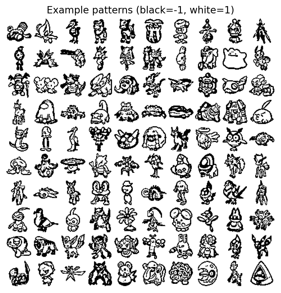
Let’s build some helper functions to load and view our data: binarized pokemon sprites. While other fields like to work with \(\{0,1\}\) binary data, Hopfield Networks like to work with bipolar data where each datapoint \(\sigma \in \{-1, 1\}^D\).
from amtutorial.data_utils import get_pokemon_datapoke_pixels, poke_names = get_pokemon_data()data = poke_pixelspxh, pxw = data.shape[-2:]data = data.reshape(-1, pxh * pxw)def gridify(images, grid_h=None):"""Convert list of images to a single grid image""" images = np.array(images) # Shape: (n_images, H*W)if grid_h isNone: grid_h =int(np.sqrt(len(images))) grid_w =int(np.ceil(len(images) / grid_h))# Pad if necessary n_needed = grid_h * grid_wiflen(images) < n_needed: padding_shape = (n_needed -len(images),) + images.shape[1:] padding = np.zeros(padding_shape) images = np.concatenate([images, padding], axis=0)# Reshape individual images and arrange in grid grid = rearrange(images[:n_needed], '(gh gw) h w -> (gh h) (gw w)', gh=grid_h, gw=grid_w)return griddef show_im(sigma, ax=None, do_gridify=True, grid_h=None, figsize=None):"""Vector to figure""" sigma = rearrange(sigma, "... (h w) -> ... h w", h=pxh, w=pxw)if do_gridify andlen(sigma.shape) ==3: sigma = gridify(sigma, grid_h) empty_ax = ax isNone figsize = figsize or (8, 2.67) # Quarto aspect ratioif empty_ax: fig, ax = plt.subplots(figsize=figsize) ax.imshow(sigma, cmap="gray", vmin=-1, vmax=1) ax.axis("off")returnNoneifnot empty_ax else fig, ax
The Classical Hopfield Network
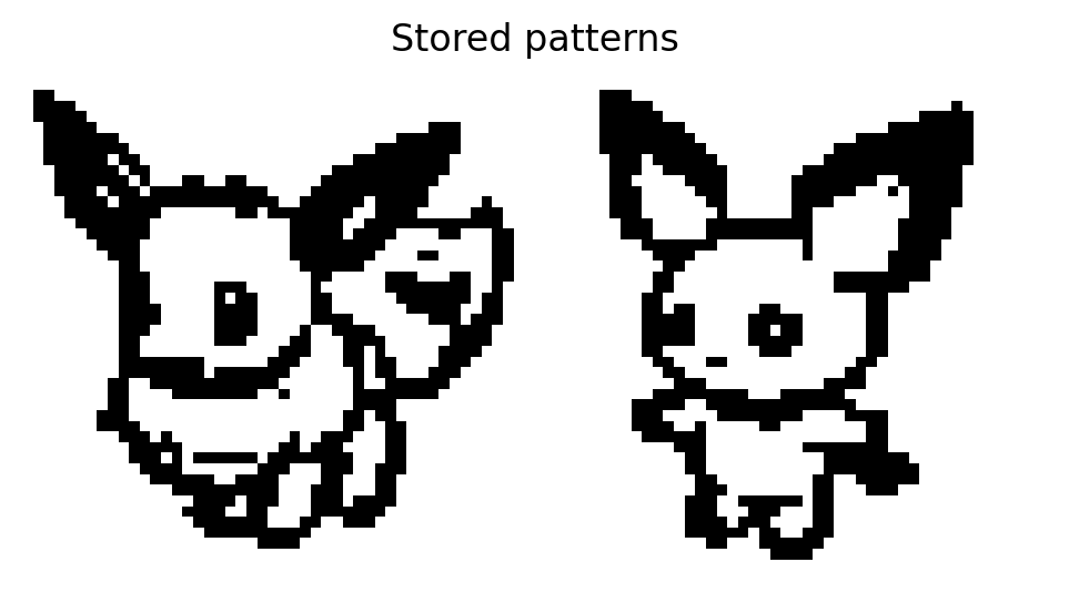
Let’s revisit our task to store \(K\) binary patterns each of dimension \(D\) into an energy function. Let’s keep things simple and fast for the first part of this notebook and focus on storing and retrieving \(K=2\) patterns: an eevee and pichu, where each (48,48) image is rasterized to a vector dimension of \(D=2304\).
desired_names = ["eevee", "pichu"]eevee_pichu_idxs = [poke_names.index(name) for name in desired_names]Xi = data[eevee_pichu_idxs]fig, ax = show_im(Xi, figsize=(6,3));ax.set_title("Stored patterns")plt.show()print(f"K={Xi.shape[0]}, D={Xi.shape[1]}")
K=2, D=2304
The Classical Hopfield Network (CHN) [1] defines an energy function for this collection of patterns, putting the \(\mu\)-th stored pattern \(\xi^\mu\) at a low value of energy. The CHN energy is a quadratic function described by dot-product correlations:
We see the familiar equation for CHN energy on the RHS if we expand the quadratic function, where \(T_{ij} := \sum_{\mu=1}^K \xi^\mu_i \xi^\mu_j\) is the matrix of symmetric synapses. Learned patterns \(\xi^\mu\) are stored in \(T\) via a simple, Hebbian learning rule.
The CHN can be easily implemented in code via
class CHN(BinaryAM):def energy(self, sigma: Float[Array, "D"] # Possibly noisy query pattern ): "Quadratic energy function for the CHN"return-0.5* jnp.sum((self.Xi @ sigma)**2, axis=0)chn = CHN(Xi)
The asynchronous update rule of Equation 1 uses the energy difference of a flipped bit to determine whether to keep the flip or not. That update rule is equivalent to the following, arguably more familiar update rule, which describes the next state based on the sign of the total input current to the neuron \(\sigma_i\).
This update rule also ensures the network always moves toward lower energy states. Because the \(E_\text{CHN}\) is bounded from below, the network will eventually converge to a local minimum that (ideally) corresponds to one of the stored patterns.
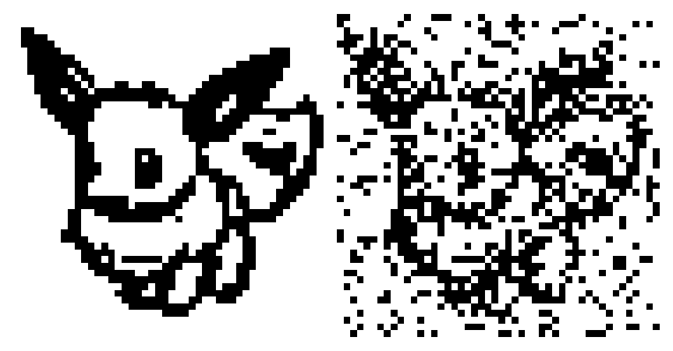
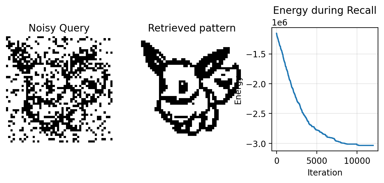
Let’s observe the recall process! We’ll start with a noisy version of the first pattern and see if we can recover it.
We can animate the recall process to view the “thinking” process of the CHN.
Retrieving “inverted” images
If we initialize a query with too much noise, it’s possible to retrieve the negative of a stored pattern or an “inverted image”. Because the energy is quadratic, both \(\sigma\) and \(-\sigma\) produce the same small value of energy. Whether we retrieve the original \(\sigma\) or the inverted \(-\sigma\) is dependent on whether we initialize our query closer to the original or inverted pattern.
Loading cached recall data
Accidentally retrieved the inverted pattern!
Memory retrieval failure
Unfortunately, the CHN is terrible at storing and retrieving multiple patterns. If we add even four more patterns into the synaptic memory, our network will fail to retrieve our eevee.
Loading cached recall data
CHN failed to retrieve the correct pattern!
Dense Associative Memory
The CHN has a quadratic energy, which is a special case of a more general class of models called Dense Associative Memory (DenseAM) [2]. If we increase the degree of the polynomial used in the energy function, we strengthen the coupling between neurons and can store more patterns into the same synaptic matrix.
The new energy function, written in terms of polynomials of degree \(n\) and using the same notation for stored patterns \(\xi^\mu_i\), is
We need \(F_n\) to be convex for all \(n\), which is why we perform the rectification. We could alternatively limit ourselves to only even values of \(n\).
Fun fact, rectified polynomials remove the “inverted” retrieval phenomenon seen in Section 1.1.
Equation 3 admits the following manual update rule for a single neuron \(i\):
Here we introduced an activation function \(f_n(\cdot) = F_n'(\cdot)\) that is the derivative of the rectified polynomial used to define the energy. This update can be viewed as the negative gradient of the energy function, ensuring that the network always moves toward lower energy states. Like before, this energy is bounded from below and we will eventually converge to a local minimum that corresponds to one of the stored patterns.
Let’s implement the DenseAM model. The primary difference from the CHN is that now we generalize the quadratic energy to a (possibly rectified) polynomial energy.
class PolynomialDenseAM(BinaryAM): Xi: jax.Array # (K, D) Memory patterns n: int# Power of polynomial F rectified: bool=True# Whether to rectify inputs to Fdef F_n(self, sims): """Rectified polynomial of degree `n` for energy""" sims = sims.clip(0) ifself.rectified else simsreturn1/self.n * sims **self.ndef energy(self, sigma): return-jnp.sum(self.F_n(self.Xi @ sigma))
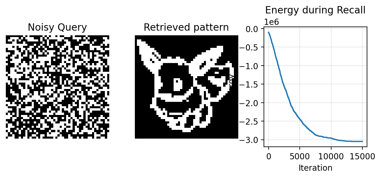
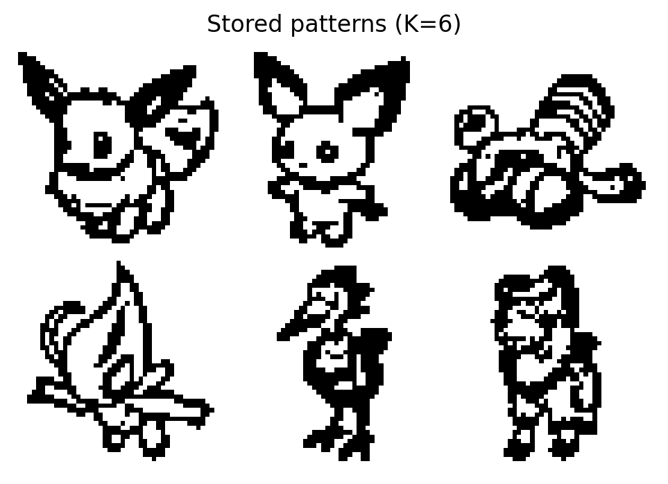
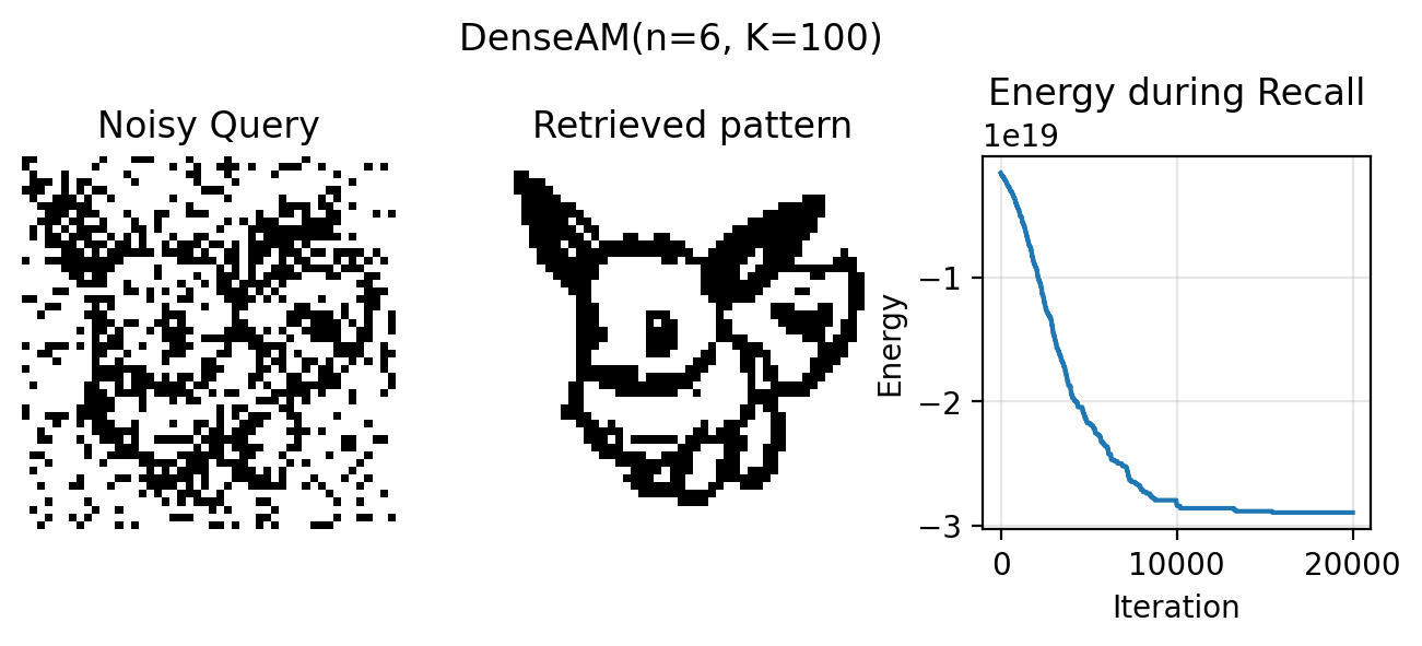
A simple change to using a polynomial of degree \(6\) instead of the CHN’s quadratic energy function allows us to store and retrieve our desired eevee even with up to \(K=100\) patterns.
A higher degree polynomial gives us more storage capacity, which means that it is easier to retrieve the patterns we have stored in the network. Note that the higher the degree \(n\), the narrower the basins of attraction, which makes it easier to pack more patterns into the energy landscape.
Gotta catch ’em all!
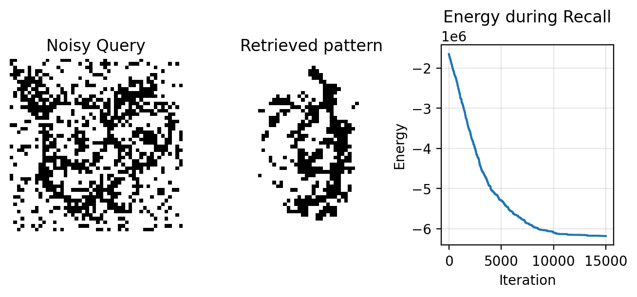
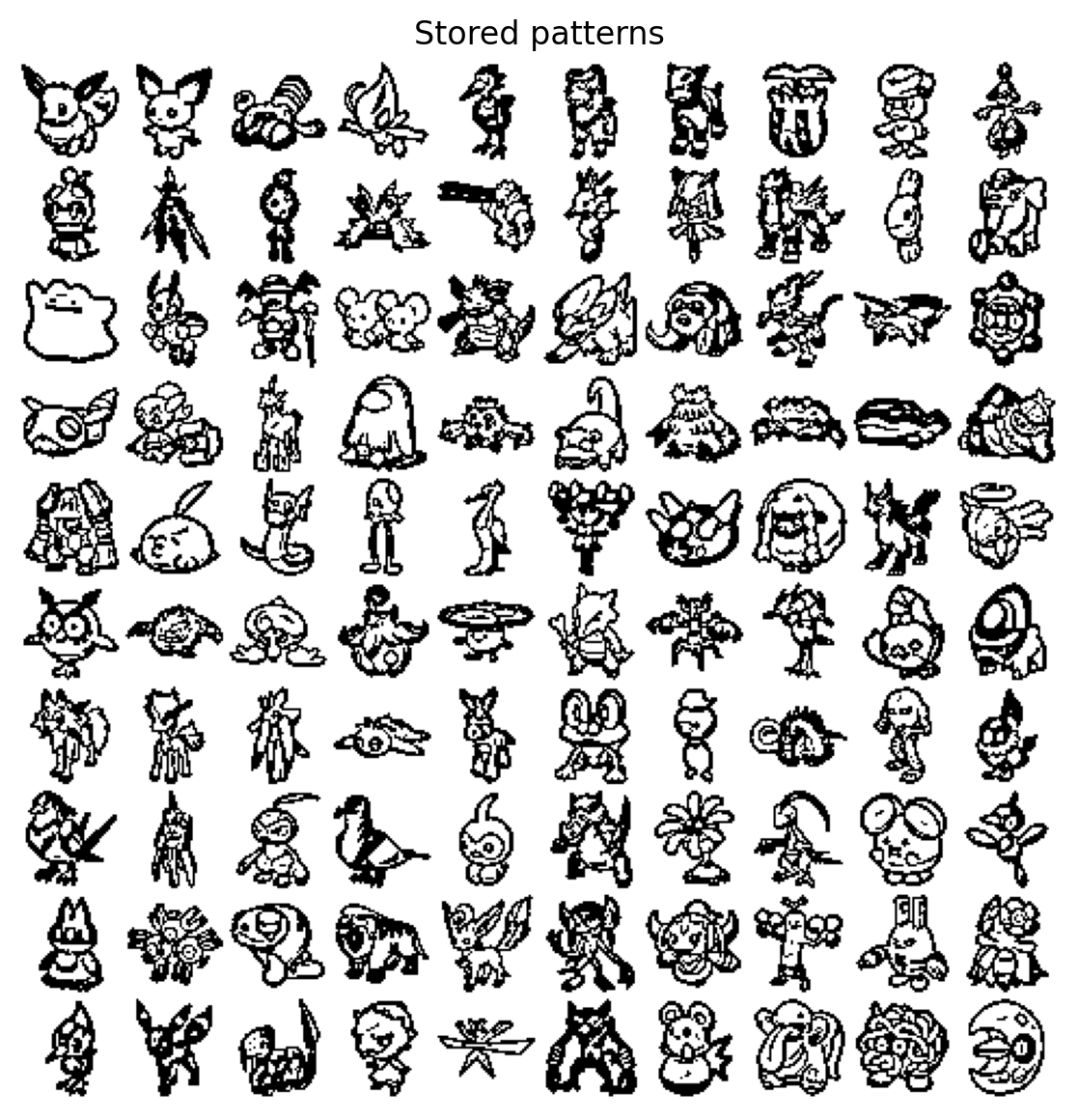
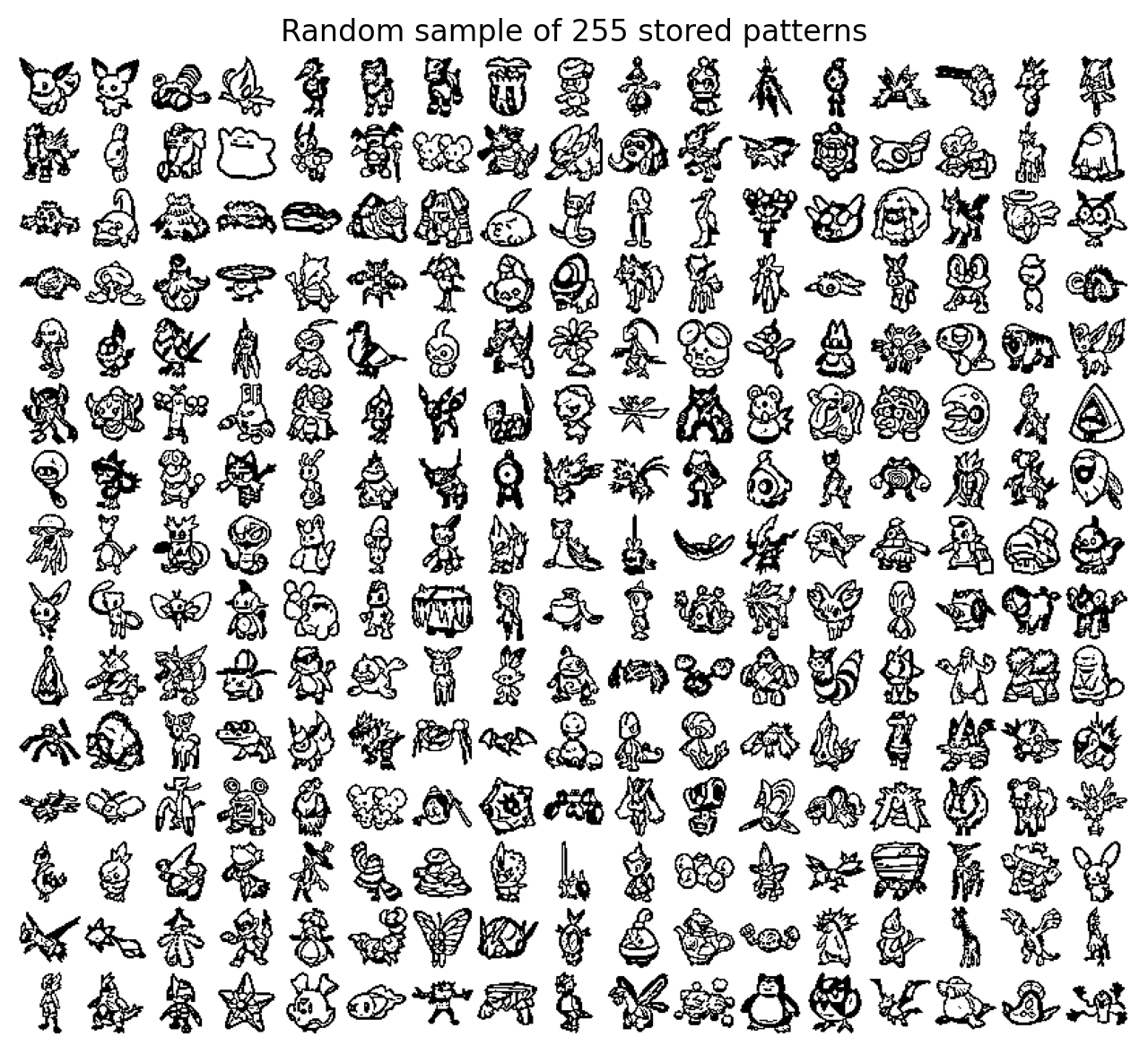
Let’s try to store and retrieve all 1024 pokemon patterns into our network (though we will only show retrieval for a subset of them for computational reasons). To do this, we’ll need very large values of \(n\), which is bad for numeric overflow (computers don’t like working in really really large numbers i.e., inf energy regimes).
We’ll implement an exponential version of the DenseAM [3]. Specifically, we will use a numerically stable logsumexp version [4].
where increasing the inverse temperature \(\beta\) has a similar effect to increasing \(n\) in the DenseAM polynomial energy function. Because the log is a monotonically increasing function, the energy minima of the original energy function are preserved, while simultaneously making the energy function more numerically stable.
class ExponentialDenseAM(BinaryAM): Xi: jax.Array # (K, D) Memory patterns beta: float=1.0# Temperature parameterdef energy(self, sigma):return-jax.nn.logsumexp(self.beta *self.Xi @ sigma, axis=-1)
Depending on your RAM availability, the following cell may crash your session. Decrease to e.g., nh = nw = 5 to avoid this (or upgrade your runtime on Colab for more resources).
And of course, what’s the fun if we can’t animate the retrieval process?
<IPython.core.display.Image object>
References
[1]
J. J. Hopfield, “Neural networks and physical systems with emergent collective computational abilities.”Proceedings of the national academy of sciences, vol. 79, no. 8, pp. 2554–2558, 1982.
[2]
D. Krotov and J. J. Hopfield, “Dense associative memory for pattern recognition,”Advances in neural information processing systems, vol. 29, 2016.
[3]
M. Demircigil, J. Heusel, M. Löwe, S. Upgang, and F. Vermet, “On a model of associative memory with huge storage capacity,”Journal of Statistical Physics, vol. 168, no. 2, pp. 288–299, May 2017, doi: 10.1007/s10955-017-1806-y.