We will train a score-based diffusion model on a small dataset of points lying on a circle. Our goal is to understand how the model learns the data distribution and to visualize its learned “energy landscape,” which reveals how it behaves like an Associative Memory system initially to later transition into a generative model.
The paper uses a simple dataset: points sampled from the circumference of a unit circle. This helps us easily visualize how the model learns.
We’ll define a function to generate these points and a PyTorch Dataset class to handle them.
def generate_circle_data(num_samples=60_000, radius=1, seed=59):"""Generates data points that lie on a unit circle.""" np.random.seed(seed)# Sample angles uniformly from 0 to 2*pi angles = np.random.uniform(0, 2* np.pi, num_samples)# Convert polar coordinates (angles, radius) to Cartesian (x, y) x = radius * np.cos(angles) y = radius * np.sin(angles)return np.stack([x, y], axis=1)class CircleDataset(Dataset):"""A PyTorch Dataset to wrap our circle data."""def__init__(self, num_samples=60_000, radius=1, seed=9):# Generate and store the data as a torch tensorself.data = torch.from_numpy(generate_circle_data(num_samples, radius, seed)).float()def__len__(self):returnlen(self.data)def__getitem__(self, idx):returnself.data[idx]def create_subset(dataset, sample_size, seed=42):"""Create a subset of the dataset based on the specified sample size. """ max_size =len(dataset) generator = torch.Generator().manual_seed(seed)ifnot1<= sample_size <=len(dataset):raiseValueError("Sample size must be between 1 and the size of the dataset inclusive.") subset, _ = torch.utils.data.random_split( dataset, [sample_size, max_size - sample_size], generator=generator )return subset
Creating a Small Training Set
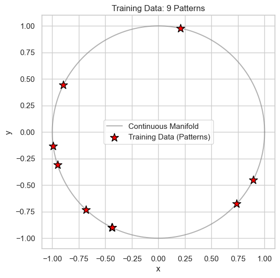
Diffusion models can learn from very few samples. In the paper, this is referred to as memorizing “patterns”. Let’s create a tiny dataset with just 9 data points (patterns) to train on.
# --- Configuration ---SAMPLE_SIZE =9# The number of data points (patterns) to memorizeBATCH_SIZE =min(500, SAMPLE_SIZE) # Use all data points in each batchSEED =9# For reproducibility# Create Datasetdataset = CircleDataset(60_000, seed=SEED)# Split Datasettrain_subset = create_subset(dataset, SAMPLE_SIZE, SEED)# Create a DataLoadertrain_loader = DataLoader(train_subset, batch_size=BATCH_SIZE, shuffle=True)# Extract the training data points for visualizationpatterns = train_subset.dataset[train_subset.indices]
Let’s plot our small dataset. These are the specific points we want our model to learn and remember.
The Diffusion Model
The diffusion model is simply a model \(s_\theta(\mathbf{x}_t, t)\) which approximates the score function: \[
s_\theta(\mathbf{x}_t, t) ≈ \nabla_{\mathbf{x}_t} \log p_t (\mathbf{x}_t)
\] over a series of timesteps.
In this tutorial, we will be using Variance Exploding (VE) SDE, which defines how data is gradually noised over time ranging from \(t \in [\epsilon, 1]\): \[
\mathrm{d} \mathbf{x}_t = \sigma \mathrm{d} \mathbf{w}_t
\] and the corresponding reverse process: \[
\mathrm{d} \mathbf{x}_t = \big [ -\sigma^2 \nabla_{\mathbf{x}_t} \log p_t (\mathbf{x}_t) \big ] \mathrm{d}t + \sigma^2 \mathrm{d} \mathbf{w}_t
\] where \(g(t) = \sigma\) is the diffusion coefficient and \(\mathbf{w}_t\) is brownian motion.
class VESDETerms:"""Defines the terms for the Variance Exploding SDE."""def__init__(self, sigma_max, device=None):self.sigma = sigma_maxself.device = devicedef marginal_prob_std(self, t): t = torch.as_tensor(t, device=self.device, dtype=torch.float32)returnself.sigma * torch.sqrt(t)def diffusion_coeff(self, t): t = torch.as_tensor(t, device=self.device, dtype=torch.float32)returnself.sigma * torch.ones_like(t)
ScoreNet Architecture
Our score network is a simple Multi-Layer Perceptron (MLP). It takes a noisy data point x and a time step t as inputs, and returns the estimated score. The conditioning on time step t is performed via the Fourier embedding, a standard method of time conditioning in diffusion models.
PyTorch ScoreNet
@torch.no_grad()def update_ema(ema_model, model, decay=0.9999):""" Step the EMA model towards the current model. """ ema_params = OrderedDict(ema_model.named_parameters()) model_params = OrderedDict(model.named_parameters())for name, param in model_params.items():if param.requires_grad ==True: ema_params[name].mul_(decay).add_(param.data, alpha=1.- decay)class FourierEmbedding(torch.nn.Module):"""Embeds time `t` into a high-dimensional feature space."""def__init__(self, embed_dim, scale=16):super().__init__()self.register_buffer('freqs', torch.randn(embed_dim //2) * scale)def forward(self, x): x = x.ger((2.* torch.pi *self.freqs).to(x.dtype)) x = torch.cat([x.cos(), x.sin()], dim=1)return xclass ScoreNet(nn.Module):"""The score-based model (a simple MLP)."""def__init__(self, input_dim=2, num_layers=4, hidden_dim=128, embed_dim=128, marginal_prob_std=None ):super().__init__()self.act = nn.SiLU()self.marginal_prob_std = marginal_prob_std# Time embeddingself.time_embed = nn.Sequential( FourierEmbedding(embed_dim=embed_dim), nn.Linear(embed_dim, embed_dim), nn.SiLU(), nn.Linear(embed_dim, embed_dim), nn.SiLU() )# Project combined (x + time-embedding) to hidden dimensionself.input_proj = nn.Linear(input_dim + embed_dim, hidden_dim)# Hidden MLP layers layers = []for _ inrange(num_layers -1): layers.append(nn.Linear(hidden_dim, hidden_dim))if _ == num_layers -2: layers.append(nn.LayerNorm(hidden_dim)) layers.append(nn.SiLU())else: layers.append(nn.SiLU())self.hidden = nn.Sequential(*layers)# Final output to 2 dimensionsself.output = nn.Linear(hidden_dim, 2)def forward(self, x, t):# Generate time embedding and concatenate with x t_emb =self.time_embed(t) h = torch.cat([x, t_emb], dim=1)# Pass through MLP h =self.input_proj(h) h =self.hidden(h) h =self.output(h)# Scale by 1 / marginal_prob_std(t)return h /self.marginal_prob_std(t)[:, None]
Training
We use the denoising score matching (DSM) loss. The goal is to train the ScoreNet model so that its output, the score, matches the direction of the noise z that was added to the clean data x at each time step t. \[
\mathcal{L} = \mathbb{E}_{\mathbf{x}_0, \mathbf{x}_t, t} \, \bigg [ \lambda(t) \lVert s_\theta (\mathbf{x}_t, t) - \nabla_{\mathbf{x}_t} \log p(\mathbf{x}_t | \mathbf{x}_0) \rVert^2 \bigg ]
\] where \(\mathbf{x}_0\) denotes the clean data point and \(\mathbf{x}_t\) is the perturbed data point.
For example, assume \(\tilde{\mathbf{x}} \sim \mathcal{N} (\tilde{\mathbf{x}} | \mathbf{x}, \sigma^2 \mathbf{I})\) for the simple case of DSM. We have the following: \[
\nabla_{\tilde{\mathbf{x}}} \log p(\tilde{\mathbf{x}} | \mathbf{x}) = \nabla_\tilde{\mathbf{x}} \bigg ( -\frac{1}{2\sigma^2} (\tilde{\mathbf{x}} - \mathbf{x})^2 \bigg ) = -\frac{\tilde{\mathbf{x}} - \mathbf{x}}{\sigma^2} = -\frac{\mathbf{z}}{\sigma}
\] as the score function, which we have to learn for a single timestep of denoising. \(\mathbf{z} \sim \mathcal{N}(0, \mathbf{I})\).
Training Loop and Loss Function
def loss_fn(model, x, marginal_prob_std, eps=1e-5):"""The denoising score matching loss function."""# Sample a random time t random_t = torch.rand(x.shape[0], device=x.device) * (1.- eps) + eps# Sample a random noise vector z = torch.randn_like(x) std = marginal_prob_std(random_t)[:, None]# Create the noisy data point perturbed_x = x + z * std# Get the model's score prediction: -z / 𝜎 score = model(perturbed_x, random_t)# Calculate the loss loss = torch.mean(torch.square(score * std + z))return lossdef train_loop(train_loader, vesde, iterations=100_000, lr=1e-4, device='cuda', log_freq=10_000):# create our score model score_model = ScoreNet(marginal_prob_std=vesde.marginal_prob_std)# create an exponential moving average version of the model ema = deepcopy(score_model).to(device) score_model = score_model.to(device)# create optimizer optimizer = torch.optim.Adam(score_model.parameters(), lr=lr)# Use an infinite data loader to cycle through our small dataset infinite_loader =iter(cycle(train_loader))# --- Training --- score_model.train() running_loss =0. pbar = tqdm(range(iterations))for iteration in pbar:# Get a batch of data x =next(infinite_loader).to(device)# Calculate loss loss = loss_fn(score_model, x, vesde.marginal_prob_std) running_loss += loss.item() loss.backward() optimizer.step() optimizer.zero_grad()# udpate ema update_ema(ema, score_model)# Log progressif iteration % log_freq ==0and iteration >0: pbar.set_description(f"Loss: {running_loss / log_freq:.4f}") running_loss =0.# return the exponential moving average model ema.eval()return ema
Time to train! The following code takes a few minutes to run, but the results are cached after the first run.
# Train our SDE-based diffusion models for training data sizes: 2, 9, and 1000.SEED =9# For reproducibilityLR =1e-4SIGMA_MAX =1.ITERATIONS =50_000# Instantiate the SDE and the Modeldevice ="cuda"if torch.cuda.is_available() else"cpu"vesde = VESDETerms(sigma_max=SIGMA_MAX, device=device)CACHE_MODELS =Truedef make_cache_name(sample_size, seed, lr, sigma_max, iterations):returnf"ema_model_{sample_size}_{seed}_{lr}_{sigma_max}_{iterations}.pth"def get_ema_model(cache_name): cache_path = CACHE_DIR / cache_nameif cache_path.exists(): model = ScoreNet(marginal_prob_std=vesde.marginal_prob_std) state_dict = torch.load(cache_path) model.load_state_dict(state_dict)return modelelse:returnNone# Will need to train itdata_sizes = [2, 9, 1000] # Takes ~5 min on an M1 Pro CPUema_set, pattern_set = [], [] # store our ema models and training patterns into two separate listsfor sample_size in data_sizes: ema =None cache_name = make_cache_name(sample_size, SEED, LR, SIGMA_MAX, ITERATIONS)# Extract the training data points for visualization batch_size =min(500, sample_size) # Use all data points in each batch train_subset = create_subset(dataset, sample_size, SEED) train_loader = DataLoader(train_subset, batch_size=batch_size, shuffle=True)if CACHE_MODELS: ema = get_ema_model(cache_name)if ema isNoneornot CACHE_MODELS: # Train the model if no cache exists torch.manual_seed(SEED) ema = train_loop(train_loader, vesde, ITERATIONS, LR, device=device) torch.save(ema.state_dict(), CACHE_DIR /f"{cache_name}") patterns = train_subset.dataset[train_subset.indices] pattern_set.append(patterns) ema_set.append(ema)
Sampling from the Trained Model
To generate new samples, we run the diffusion process in reverse. We start with pure random noise (sampled at t=1) and use our trained score model to guide it back towards the data distribution (towards t=0). This is done using a numerical SDE solver, like the Euler-Maruyama method.
Euler-Maruyama Sampler
def Euler_Maruyama_sampler(score_model, sde, batch_size=64, num_steps=1000, device='cuda', eps=1e-5):"""Generate samples from the score-based model using the Euler-Maruyama solver.""" score_model.eval() t_end = torch.ones(batch_size, device=device)# Start with orthogonalized random noise ~ N(0, sigma_max^2 * I) init_x = torch.randn(batch_size, 2, device=device) init_x = init_x / torch.norm(init_x, dim = (1), keepdim=True) init_x = init_x * sde.marginal_prob_std(t_end)[:, None] time_steps = torch.linspace(1., eps, num_steps, device=device) step_size = time_steps[0] - time_steps[1] #dt x = init_xwith torch.no_grad():for time_step in tqdm(time_steps, desc="Sampling"): batch_time_step = torch.ones(batch_size, device=device) * time_step g = sde.diffusion_coeff(batch_time_step)# This is the reverse SDE update step mean_x = x + (g**2)[:, None] * score_model(x, batch_time_step) * step_size eps = torch.randn_like(x) noise = torch.sqrt(step_size) * g[:, None] * eps x = mean_x + noise score_model.train()return mean_x # Return the final denoised sample
We can now sample from the trained models.
Sampling from the Trained Models
generated_set = []for ema in ema_set: generated_samples = Euler_Maruyama_sampler(ema, vesde, batch_size=1_500, device=device) generated_samples = generated_samples.detach().cpu().numpy() generated_set.append(generated_samples)
Potential Energy of Generated and Data Samples
Recall the relationship between energy and probability denoted by the Boltzmann distribution: \[
p_\theta(\mathbf{x}) = \frac{\exp{(-E_\theta(\mathbf{x}))} }{Z_\theta}
\] This indicates that our energy (up to a constant) is obtained by computing the negative log-likelihood: \[
-\log p_\theta(\mathbf{x}) = E_\theta(\mathbf{x}) + C
\]
Since we are dealing with a non-equilibrium system, that is our diffusion model, we follow the formulations and codes provided in Song et al. (2021) to compute the log-likelihood: \[
\log p_0(\mathbf{x}_0;\mathbf{\theta}) = \log p_T(\mathbf{x}_T; \theta) + \int_0^T \nabla \cdot \tilde{\mathbf{f}}(\mathbf{x}_t, t) \mathrm{d}t
\] where \[
\tilde{\mathbf{f}}(\mathbf{x}_t, t) =-\frac{1}{2}\sigma^2 \nabla_{\mathbf{x}_{t}} \log p_t(\mathbf{x}_{t}; \theta)
\] for this setting. Keep in mind, \(\nabla \cdot ()\) denotes the laplacian operation.
To derive the above equation, we start with the Fokker-Planck equation, as did in Chen et al. (2018) and Song et al. (2021), which yields the following general probability flow ODE (derived from the forward process SDE): \[
\mathrm{d} \mathbf{x}_t = \tilde{\mathbf{f}}(\mathbf{x}_t, t)\mathrm{d} t + \tilde{\mathbf{g}} (\mathbf{x}_t, t) \mathrm{d} \mathbf{w}_t
\] where \[\tilde{\mathbf{f}}(\mathbf{x}_t, t) = \mathbf{f} (\mathbf{x}_t, t) - \frac{1}{2} \nabla \cdot \big[\mathbf{g} (\mathbf{x}_t, t) \mathbf{g} (\mathbf{x}_t, t)^\top \big] - \frac{1}{2} \big [ \mathbf{g} (\mathbf{x}_t, t) \mathbf{g} (\mathbf{x}_t, t)^\top \big ] \nabla_{\mathbf{x}_t} \log p_t(\mathbf{x}_t)\] and \(\tilde{\mathbf{g}} (\mathbf{x}_t, t) = 0\).
Here, \(\mathbf{f}(\mathbf{x}_t, t) = 0\) denotes the drift term which vanishes in the VE setting while \(\mathbf{g} (\mathbf{x}_t, t) = \sigma\) which is constant in this setting. Thus, the probability flow ODE for our setting is simply: \[
\mathrm{d} \mathbf{x}_t = \tilde{\mathbf{f}}(\mathbf{x}_t, t)\mathrm{d} t = -\frac{1}{2}\sigma^2 \nabla_{\mathbf{x}_{t}} \log p_t(\mathbf{x}_{t}) \, \mathrm{d}t
\]
Computing the Laplacian and Log-Likelihood
# @title Code to Compute Laplacian and Log-Likelihooddef compute_laplacian(score_fn, x, t):""" Compute the Laplacian of the score function using torch.func utilities. This is a more efficient, vectorized alternative to the loop-based approach. """def get_laplacian_for_single_sample(x_sample, t_sample):""" A helper function that computes the Laplacian for one sample. This is the function we will vectorize using vmap (like Jax). """# We have to unsqueeze since torch module requires a batch dim. f =lambda x_inp: score_fn(x_inp[None], t_sample[None]).squeeze(0)# Compute the Jacobian of the score function w.r.t. x.# This gives a D x D matrix where D is the dimension of x. J = torch.func.jacrev(f)(x_sample)# The Laplacian is the trace of the Jacobian matrix (sum of its diagonal).return torch.trace(J)# Apply vmap over the first dimension for both inputsreturn torch.func.vmap(get_laplacian_for_single_sample, in_dims=(0, 0))(x, t)def ode_likelihood_with_laplacian(x, score_model, sde, device='cuda', eps=1e-5):"""Compute the log-likelihood of x by solving the probability flow ODE.""" shape = x.shapedef score_eval_wrapper(sample, time_steps):"""A wrapper for evaluating the score-based model for the ODE solver.""" sample = torch.tensor(sample, device=device, dtype=torch.float32).reshape(shape) time_steps = torch.tensor(time_steps, device=device, dtype=torch.float32).reshape((sample.shape[0], ))with torch.no_grad(): score = score_model(sample, time_steps)return score.cpu().numpy().reshape((-1, shape[1])).astype(np.float64)def laplacian_eval_wrapper(sample, time_steps):"""A wrapper for evaluating the Laplacian of the score function.""" sample = torch.tensor(sample, device=device, dtype=torch.float32).reshape(shape) time_steps = torch.tensor(time_steps, device=device, dtype=torch.float32).reshape((sample.shape[0], )) laplacian = compute_laplacian(score_model, sample, time_steps)return laplacian.cpu().numpy().reshape((-1,)).astype(np.float64)def ode_func(t, x_and_logp): time_steps = torch.from_numpy(np.ones((shape[0],)) * t).to(device, torch.float32) sample = torch.from_numpy(x_and_logp[:-shape[0]].reshape(shape)).to(device, torch.float32)with torch.no_grad(): g = sde.diffusion_coeff(time_steps).cpu().numpy() score = score_eval_wrapper(sample, time_steps) laplacian = laplacian_eval_wrapper(sample, time_steps) drift =-0.5* g[:, None]**2* score logp_grad =-0.5* g**2* laplacianreturn np.concatenate([drift.flatten(), logp_grad], axis =0) init = np.concatenate([x.cpu().numpy().flatten(), np.zeros((shape[0],))]) res = integrate.solve_ivp(ode_func, (eps, 1.), init, rtol=1e-5, atol=1e-5, method='RK45') zp = torch.tensor(res.y[:, -1], device=device) z = zp[:-shape[0]].reshape(shape) delta_logp = zp[-shape[0]:] sigma_max = sde.marginal_prob_std(torch.tensor(1.)) prior_logp =-shape[1] /2.* torch.log(2* np.pi * sigma_max **2) prior_logp = prior_logp - torch.sum(z **2, dim=-1) / (2* sigma_max **2)return (prior_logp + delta_logp)
Visualizing the Energy
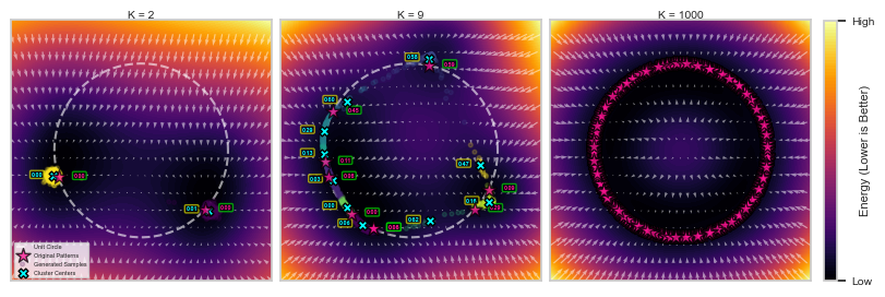
Since we are generating quite a lot of synthetic data points, we use hierarchical clustering to get a sense of where the concentrations of these new points are at. To be more informative, we are also displaying the energy profile of these concentrations alongside that of the training data points.
At K = 2, we can see that the concentrations of generated points are pretty much surrounding the data points and their energy profile are similar to that of the training data points.
Meanwhile, at K = 9, we now see local minima of the energy that devitate drastically from the training points. These new local minima of the energy are called spurious patterns.
Finally, when K = 1000, the energy now very closely matches that of the DenseAM’s derived exact energy, see below.
Plot Functions for Energy Landscape in 2D and 3D
# @title Plot Functions for Energy Landscape in 2D and 3Ddef to_energy(loglikelihood, normalize=True):# nll = E + C energy =-loglikelihoodif normalize:# normalize energy by its minimumreturn energy - energy.min()return energydef plot_combined_landscape(fig, ax, score_model, sde, patterns, samples, labels, centers, t_eval=1e-5, device='cpu', annotate=True, quiver_stride=10):"""Visualize the energy landscape with annotated points.""" score_model.eval()# 1. Calculate Energy for Patterns and Centers# Energy for original patterns patterns_tensor = patterns.to(device) logp_patterns = ode_likelihood_with_laplacian(patterns_tensor, score_model, sde, device, eps=t_eval) energy_patterns = to_energy(logp_patterns).cpu().numpy()# Energy for found cluster centers centers_tensor = torch.from_numpy(centers).float().to(device) logp_centers = ode_likelihood_with_laplacian(centers_tensor, score_model, sde, device, eps=t_eval) energy_centers = to_energy(logp_centers).cpu().numpy()# 2. Create a grid of points bounds=(-1.5, 1.5); resolution=75 x_ = torch.linspace(bounds[0], bounds[1], resolution) y_ = torch.linspace(bounds[0], bounds[1], resolution) X, Y = torch.meshgrid(x_, y_, indexing='ij') grid_tensor = torch.stack([X.flatten(), Y.flatten()], dim=1).to(device)# 3. Calculate the energy and score for the grid logp_grid = ode_likelihood_with_laplacian(grid_tensor, score_model, sde, device, eps=t_eval) energy_grid = to_energy(logp_grid).cpu().numpy().reshape(resolution, resolution)with torch.no_grad(): vec_t = torch.ones(grid_tensor.shape[0], device=device) * t_eval scores = score_model(grid_tensor, vec_t).cpu().numpy()# 4. Create the comprehensive plot ax.set_title(f'K = {len(patterns)}', fontsize=7.5, pad=-0.025) ax.set_aspect('equal'); ax.grid(False)# Plot energy contour contour = ax.contourf(X.cpu(), Y.cpu(), energy_grid, levels=100, cmap='inferno', zorder=0)# Plot the unit circle theta = np.linspace(0, 2* np.pi, 200) ax.plot(np.cos(theta), np.sin(theta), color='white', linestyle='--', alpha=0.6, zorder=1, label='Unit Circle')# Plot score field ax.quiver(grid_tensor[:, 0].cpu()[::quiver_stride], grid_tensor[:, 1].cpu()[::quiver_stride], scores[:, 0][::quiver_stride], scores[:, 1][::quiver_stride], color='white', alpha=0.5, width=0.005, headwidth=3, zorder=2)# Plot original patterns ax.scatter(patterns[:, 0].cpu(), patterns[:, 1].cpu(), marker="*", alpha=0.75, s=100, color="deeppink", label="Original Patterns", edgecolor='black', zorder=5)if annotate: # turn off annotation and plotting center since there are too many patterns at this point# Plot generated samples ax.scatter(samples[:, 0], samples[:, 1], c=labels, cmap='viridis', s=7.5, alpha=0.2, zorder=3, label='Generated Samples')# Plot found cluster centers ax.scatter(centers[:, 0], centers[:, 1], marker='X', s=40, color='aqua', edgecolor='black', zorder=4, label='Cluster Centers')# Add energy annotations for patternsfor i, p inenumerate(patterns.cpu().numpy()): ax.annotate(f'{energy_patterns[i]:.2f}', (p[0], p[1]), xytext=(10, 0), textcoords='offset points', color='deeppink', fontsize=4, weight='bold', bbox=dict(boxstyle="round,pad=0.2", fc="black", ec="lime", lw=1, alpha=0.6))# Add energy annotations for cluster centersfor i, c inenumerate(centers): ax.annotate(f'{energy_centers[i]:.2f}', (c[0], c[1]), xytext=(-15, 0), textcoords='offset points', color='aqua', fontsize=4, weight='bold', bbox=dict(boxstyle="round,pad=0.2", fc="black", ec="yellow", lw=1, alpha=0.6))#ax.set_xlabel('x', fontsize=5.5); ax.set_ylabel('y', fontsize=5.5); ax.set_xticks([]); ax.set_yticks([]); ax.set_xlim(bounds); ax.set_ylim(bounds);return contourdef plot_energy_surface_3d(fig, ax, X, Y, energy, view_angle=(60, -60), title=None):""" Creates a 3D surface plot of the energy landscape. Args: X (np.ndarray): Meshgrid for X coordinates. Y (np.ndarray): Meshgrid for Y coordinates. energy (np.ndarray): 2D array of energy values. view_angle (tuple): Tuple of (elevation, azimuth) for the plot's camera angle. """# Plot the 3D surface surface = ax.plot_surface(X, Y, energy, cmap='inferno', rstride=1, cstride=1, linewidth=0, antialiased=True, alpha=0.9)# Set labels and title ax.set_xlabel('x', fontsize=5, labelpad=-18) ax.set_ylabel('y', fontsize=5, labelpad=-18) ax.set_zlabel('Energy', fontsize=5, labelpad=-18, rotation=-90) ax.set_title(title, fontsize=7.5, y=-0.08) ax.set_xticks([]) ax.set_yticks([]) ax.set_zticks([])# Set a nice viewing angle ax.view_init(elev=view_angle[0], azim=view_angle[1])return surface
Visualization of the Energy Landscape Across K training Sizes in 2D
# This threshold determines how close points need to be to be considered in the same cluster.# You may need to tune this value based on your results.dist_thresholds = [3, 2, 0.45]annotates = [True, True, False]t_evals = [0.15] *len(dist_thresholds) # evaluate potentials at eps = 0.15fig, axs = plt.subplots(1, 3, figsize=(8, 8), constrained_layout=True)for i, (patterns, generated_samples, ema, threshold, t_eval, annotate) inenumerate(zip(pattern_set, generated_set, ema_set, dist_thresholds, t_evals, annotates)):# Perform Agglomerative (Hierarchical) Clustering clustering = AgglomerativeClustering( n_clusters=None, # We let the algorithm find the clusters based on the threshold distance_threshold=threshold ).fit(generated_samples)# Find the center of each identified cluster cluster_labels = clustering.labels_ n_clusters_found =len(np.unique(cluster_labels)) cluster_centers = np.array([ generated_samples[cluster_labels == i].mean(axis=0)for i inrange(n_clusters_found) ]) contour = plot_combined_landscape( fig, axs[i], ema, vesde, patterns, generated_samples, cluster_labels, cluster_centers, device=device, t_eval=t_eval, annotate=annotate, )axs[0].legend(loc='lower left', fontsize=4)# Set the ticks to only be at the min and maxcbar = fig.colorbar(contour, ax=axs[-1], shrink=0.3)cbar.set_label('Energy (Lower is Better)', fontsize=8, labelpad=-10)vmin, vmax = contour.get_clim()cbar.set_ticks([vmin, vmax])cbar.set_ticklabels(['Low', 'High'], fontsize=7.5)plt.show()
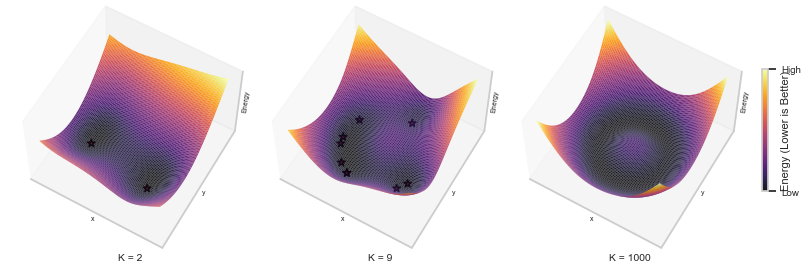
Visualization of the Energy Landscape Across K training Sizes in 3D
# This code is slow to run, so we cache the figureCACHE_FIG =Truebounds = (-1.5, 1.5)resolution =100X_grid, Y_grid = torch.meshgrid( torch.linspace(bounds[0], bounds[1], resolution), torch.linspace(bounds[0], bounds[1], resolution), indexing='ij')grid_tensor = torch.stack([X_grid.ravel(), Y_grid.ravel()], dim=1).to(device)fig_fname = CACHE_DIR /"slow_fig.png"if CACHE_FIG and fig_fname.exists(): img = Image.open(str(fig_fname)) display(img)else: fig, axs = plt.subplots(1, 3, figsize=(8, 6), constrained_layout=True, subplot_kw={"projection": "3d"})for i, (patterns, score_model, annotate, eps) inenumerate(zip(pattern_set, ema_set, annotates, t_evals)):# Calculate the energy for the grid (this is the slow step) logp_grid = ode_likelihood_with_laplacian(grid_tensor, score_model, vesde, device=device, eps=eps) energy_grid = to_energy(logp_grid).cpu().numpy() energy_grid = energy_grid.reshape(resolution, resolution)# Create the plot contour = plot_energy_surface_3d(fig, axs[i], X_grid.cpu().numpy(), Y_grid.cpu().numpy(), energy_grid, title=f'K = {len(patterns)}')# show the data points again...if annotate: axs[i].scatter( patterns[:, 0].cpu(), patterns[:, 1].cpu(), marker="*", alpha=0.75, s=35, color="deeppink", label="Original Patterns", edgecolor='black', zorder=5 )# Set the ticks to only be at the min and max cbar = fig.colorbar(contour, ax=axs[-1], shrink=0.25) cbar.set_label('Energy (Lower is Better)', fontsize=8, labelpad=-15) vmin, vmax = contour.get_clim() cbar.set_ticks([vmin, vmax]) cbar.set_ticklabels(['Low', 'High'], fontsize=7) plt.savefig(fig_fname)plt.show()
Exact Energy from Dense Associative Memory
Consider the typical DenseAM’s energy function which involves the logsumexp function: \[
E^\text{AM}(\mathbf{x}) = -\beta^{-1} \log \bigg[\sum\limits_{\mu=1}^K \exp\Big(- \beta \lVert \mathbf{x} - \boldsymbol{\xi}^\mu \rVert^2_2\Big) \bigg]
\] which is related to the energy of the diffusion model, derived in our work: \[
E^\text{DM}(\mathbf{x}_t, t) = -2 \sigma^2 t \log\bigg[\sum\limits_{\mu=1}^K \exp \Big(- \frac{\lVert \mathbf{x}_t - \boldsymbol{\xi}^\mu \rVert^2_2}{2 \sigma^2 t}\Big) \bigg]
\]
Both of these energies expressed competitions among the memories (or stored data patterns). But, the main difference is in the value of the inverse temperature\(\beta\). In the case of diffusion models, it is alternating over time, i.e., \(\beta_t = \frac{1}{2 \sigma^2 t}\), but for DenseAM, this variable is fixed. Nonetheless, although their dynamical trajetories are slightly different, the fixed points (obtained at \(t \approx 0\)) of both equations are still the same.
Using DenseAM energy, for the case of \(K = 2\), we have the following: \[
E^\text{AM}(\mathbf{x}) = -\beta^{-1} \log \Big[\exp \Big(- \beta \lVert \mathbf{x} - \boldsymbol{\xi}^1 \rVert^2_2\Big) + \exp \Big(- \beta \lVert \mathbf{x} - \boldsymbol{\xi}^2 \rVert^2_2 \Big) \Big]
\]
For small finite values of \(\beta\), it is possible for a minimum to exist: \[
\boldsymbol{\eta} = \underset{\mathbf{x}}{\text{arg min}} \, E^\text{AM}(\mathbf{x})
\] such that \(\boldsymbol{\eta} \neq \xi^1\) and \(\boldsymbol{\eta} \neq \xi^2\). This minimum is the spurious pattern.
Assume that the empirical data distribution is \(p(\mathbf{y}) = \frac{1}{K}\sum\limits_{\mu=1}^K \delta^{(N)}(\mathbf{y} - \boldsymbol{\xi}^\mu)\) where \(\boldsymbol{\xi}^\mu\) represents an individual data point (with data size \(K\)).
When the training data size \(K \rightarrow \infty\), this empirical data distirbution becomes a continuous density of states: \[
p(\mathbf{y}) = \frac{1}{\pi} \delta\big(y_1^2+y_2^2-1\big)
\] The probability of the generated data is then proportional (up to terms independent of the state \(\mathbf{x}\)) to \[
p(\mathbf{x}) \sim \int\limits_{-\infty}^{+\infty} dy_1 dy_2\ p(\mathbf{y})\ e^{- \beta \lVert \mathbf{x} - \mathbf{y} \rVert^2_2} = e^{-\beta (R^2+1)} I_0(2\beta R)
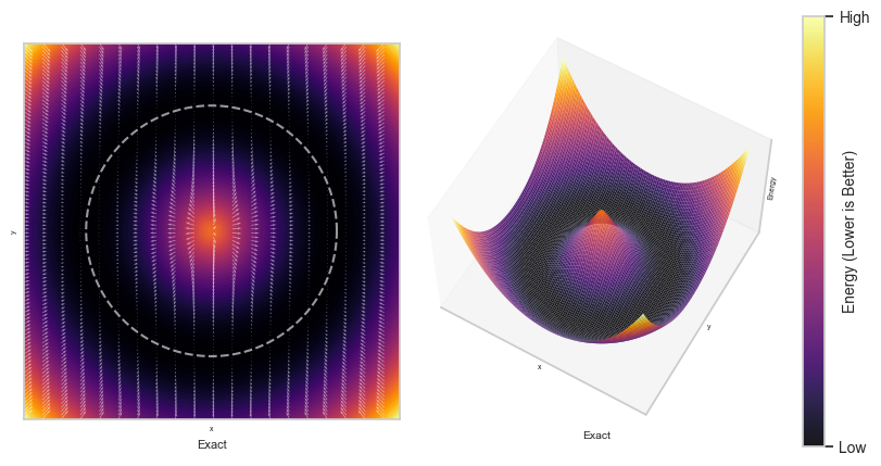
\] where \(I_0(\cdot)\) is a modified Bessel function of the first kind and \(R\) is the radius of the circle. Then, the exact energy of our toy model is the following: \[
E^\text{AM}(R, \phi) = R^2+1 - \frac{1}{\beta} \log\big[I_0(2\beta R)\big] \underset{\beta\rightarrow\infty}{\approx} (R - 1)^2
\] given the polar angle \(\phi\).
The Empirical Energy and Score Function for the Toy Model
def cartesian_to_polar(samples): x, y = samples[:, 0], samples[:, 1] r = np.sqrt(x **2+ y **2) angles = np.arctan2(y, x)return r, anglesdef energy_am(samples, beta, normalize=True):""" Computes the energy function E^AM(R, phi) = R^2 + 1 - (1 / beta) * log(I_0(2 * beta * R)) See Eq. (13) in the paper. """ r, _ = cartesian_to_polar(samples) energy = r**2+1- (1/ beta) * np.log(i0(2* beta * r))# Shift so that the lowest energy isif normalize: energy = energy - energy.min()return energydef score_am(samples, beta, epsilon=1e-6):""" Computes the score function S^AM(R, phi) = -2 * R - (2 / beta) * I_1(2 * beta * R) / I_0(2 * beta * R) See Eq. (18) in the paper. """ r, _ = cartesian_to_polar(samples)# Ensure r is not zero to avoid division by zero r = np.clip(r, epsilon, np.inf) bessel_ratio = i1(2* beta * r) / i0(2* beta * r) score_r =2* (bessel_ratio - r) score = score_r[:, None] * samples / r[:, None]return score
Visualization of the Empirical Energy Landscape and its Score Function